This is part one of our two-part data assimilation series. Part two is accessible here.
For ships at sea and coastal communities, having accurate weather and wave forecasts is critical. At Sofar, we are using the real-time ocean observations recorded by our global network of Spotter buoys to improve the traditional, open source forecast models used by organizations like NOAA.
Traditional wave forecasts use information about what the waves are like today and some rules about how waves typically behave to predict what the waves will be like tomorrow. This is an imperfect approach, partially because we do not have a perfect understanding of the world and how waves will behave. In fact, our knowledge about today's waves is mostly based on a model informed by yesterday's wave conditions!
To improve upon traditional models, we need more information about the current wave conditions across the globe. With this added information, we can then start to better predict what the wave conditions will be tomorrow and beyond.
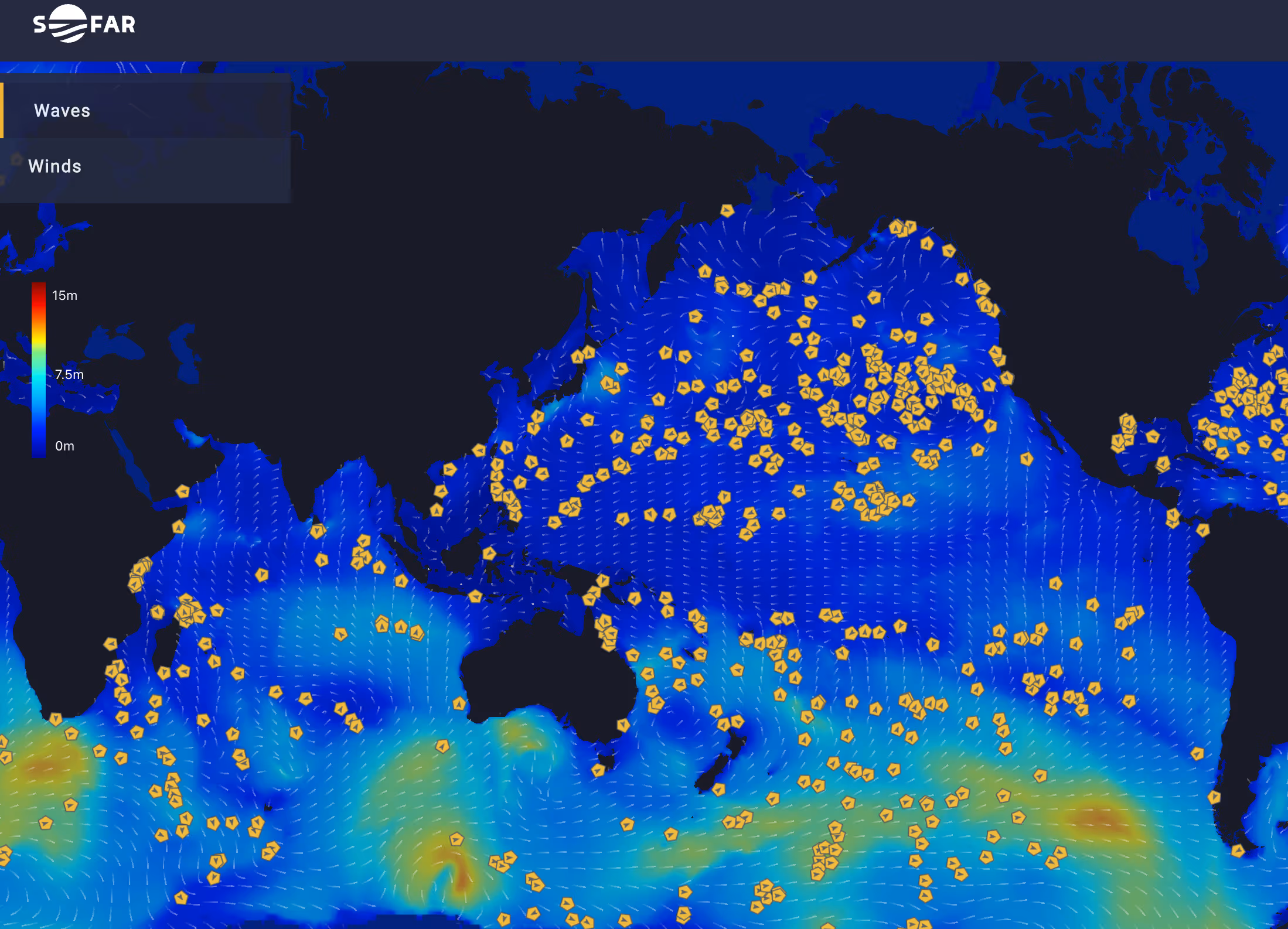
Luckily, Sofar collects over 13,500 observations of significant wave height every day. We gather this information using Spotter buoys that measure a variety of ocean variables, including wave height, sea surface temperature, and air pressure while drifting with the ocean currents. The buoys communicate with the Sofar team via satellite every hour, sharing valuable information about the ocean. Sofar’s team of scientists then uses the data collected by Spotter buoys to improve wave forecasts.
Using Spotter wave observations to update the initial conditions of computer models is called data assimilation. This methodology is what makes Sofar’s forecasts stand out.
Sofar has been assimilating Spotter measurements of significant wave height to initialize our operational wave forecasts since December 2019, an effort that has improved the accuracy of both our best guess of current wave conditions as well as forecasts several days into the future (Smit, et al., 2020).
We can visualize the data assimilation process using the animation in Figure 1 of buoys floating on the ocean surface. Sometimes, the model and the buoy will measure the same wave height, as is the case with the buoy on the left. However, other times the buoy will not agree with the model, as is the case with the buoy on the right (Step 1). When there is a discrepancy, we make an adjustment to our best guess of the current wave conditions. In this example, we increase the estimated wave height, bringing it closer to the observed value (Step 2). This ultimately creates a new model initial state that we use as the best guess of current wave conditions in our operational wave forecast (Step 3).

In Figure 1, we use the sea surface height as an analog for how we assimilate Spotter buoy data. In practice, we model the significant wave height, which is not a single wave that you can see, but the average of the largest third of the wave heights observed in the course of 30 minutes. This gives us one representative value of how big the waves are. In reality, at an individual moment, the sea surface could be bigger or smaller than the significant wave height. As a rule of thumb, the maximum wave height can be estimated as two times the significant wave height measured. So, if the buoy reports a 10 ft significant wave height, then the maximum individual wave height out at sea could be as high as 20 ft tall!
Significant wave height is a critical metric, but it tells an incomplete story about a wave’s behavior. With this in mind, the Sofar team has developed a new and unique approach to data assimilation for wave forecasts (Houghton et al., 2022). Because Spotters also collect information about the period and direction of waves, the Sofar team can separate different types of waves, rather than just take a snapshot of all waves at a single location and time.
Let’s imagine two different sea states, visualized below in Figure 2, that have similar significant wave heights, but very different wave periods. On the left are waves generated by winds: these high frequency waves have short periods and, if you were out on a boat, you would see white capping in a wind sea. The sea would appear quite chaotic, with waves moving generally in the direction of the wind.
On the right, far from the wind sea, swell waves are depicted. Swell waves are long period waves that are generated during storms and travel great distances. We often visualize swell waves by picturing a surfer trying to ride them as they crash upon the shore. Even though the wave heights are similar on the left and the right, the sea states are quite different.
[Read More: Spotter Data Partitioning for “sea” and “swell”]

In Figure 2, the directions of the waves are also distinct. In the wind sea on the left, it would be hard to tell which direction the waves were traveling; in the swell on the right, the wave direction would be apparent. Measuring direction is critical because if there’s a storm, we want to know which way the waves are propagating. Like watching ripples in a pond, we want to accurately predict how waves will travel outwards and impact nearby regions and coastlines. Ships at sea are particularly interested in predicting swell waves to understand vessel motion, as the size and direction of a swell affects how a ship rocks.
Recently, Sofar updated its data assimilation method to incorporate this critical wave direction and period information. We use a new approach where spectral wave information — the energy distribution at many different wave frequencies — is incorporated into the model at regular intervals to improve the forecast accuracy. Instead of just raising or lowering the significant wave height in the model to match that recorded by the Spotter buoys (see Figure 1), we might also lengthen the waves in the model to become more representative of an ocean swell or adjust the wave direction to improve downstream impacts in the forecasts. On the other hand, spectral data assimilation may reduce wave periods, making the model more representative of a wind sea.
In Figure 3 below, our Spotter buoy network observes waves with greater wave heights and shorter periods than the model predicted (Step 1). As a result, the spectral data assimilation approach decreases the wavelengths and increases the wave heights in the model, bringing them closer to observed values (Step 2). This ultimately creates a new model initial state that we use as the best guess of current wave conditions in our operational wave forecast (Step 3).

Now that we’ve walked through the basics of data assimilation and detailed how Sofar is incorporating spectral wave information to improve forecast accuracy, it’s time for part two of our data assimilation series, in which we take a look at a real-world example — access it here.
References:
I. A. Houghton et al., (2022). Operational Assimilation of Spectral Wave Data From the Sofar Spotter Network. Geophysical Research Letters https://doi.org/10.1002/essoar.10511124.1
P. B. Smit et al., (2020). Assimilation of distributed ocean wave sensors. Ocean Modelling, 159. https://www.sciencedirect.com/science/article/pii/S1463500320302407
Updated May 26, 2022


.jpg)
%20(1).JPG)