Sound is the most data-hungry measurement a Spotter makes. A water temperature reading is transmitted as a single integer, which we pack into 20 bits. A dissolved oxygen reading can be packed into just 17 bits. A single minute of raw audio from a hydrophone can hold more data than months of those readings.
Spotters often work in coastal waters with no cellular coverage, so satellite is the only way to transmit data home, and data transmission via satellite is priced by how much you send. You can't send everything. So the real engineering problem behind Spotter Sound isn't capturing sound. It's deciding, at every step, what is worth the cost of sending.
Our answer is a pipeline built in layers, each sending as much detail as the connection can afford: compact statistics over satellite, higher resolution data over cellular, and the full recording kept on the device.
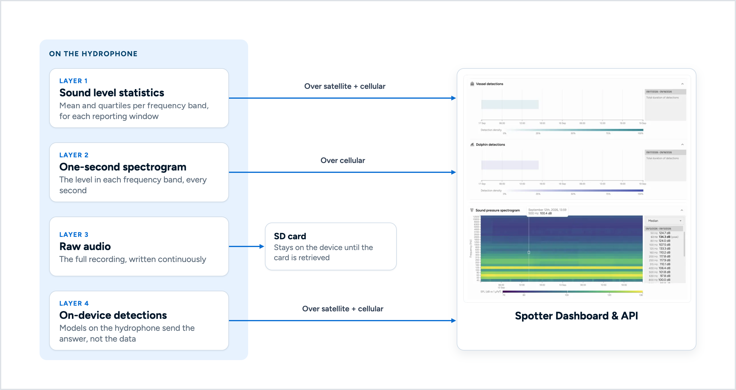
Every Spotter includes a satellite modem, which sends the most compact layer: a set of aggregated statistics. The hydrophone summarizes sound in reporting windows, fixed stretches of time. For each window, it calculates the sound pressure level (SPL) in each of a set of frequency bands, known as band levels, along with statistics that describe how those levels varied.
Why more than an average? Because an average hides too much: a window with a soft, steady hum and a quiet window with one loud vessel passing can look much the same. So alongside the mean in each band we send the quartiles: the 25th, 50th (median) and 75th percentiles. They aren't designed to tell you the exact moment when a vessel passed, but they show that the window wasn't uniform, and which frequency bands were affected.
Even that is large compared with a temperature or dissolved oxygen reading, so we round levels to steps of 0.75 dB, about 30 times coarser than the one-second readings described below, which makes the message much smaller once compressed. It's a deliberate trade: a little precision for a message that's affordable to send over satellite, every window, for the life of the deployment.
The result is coarse but continuous: the baseline loudness of a place and its daily rhythms, like a port that gets loud with activity every morning at nine. To see what happens inside a window, you need more bandwidth.
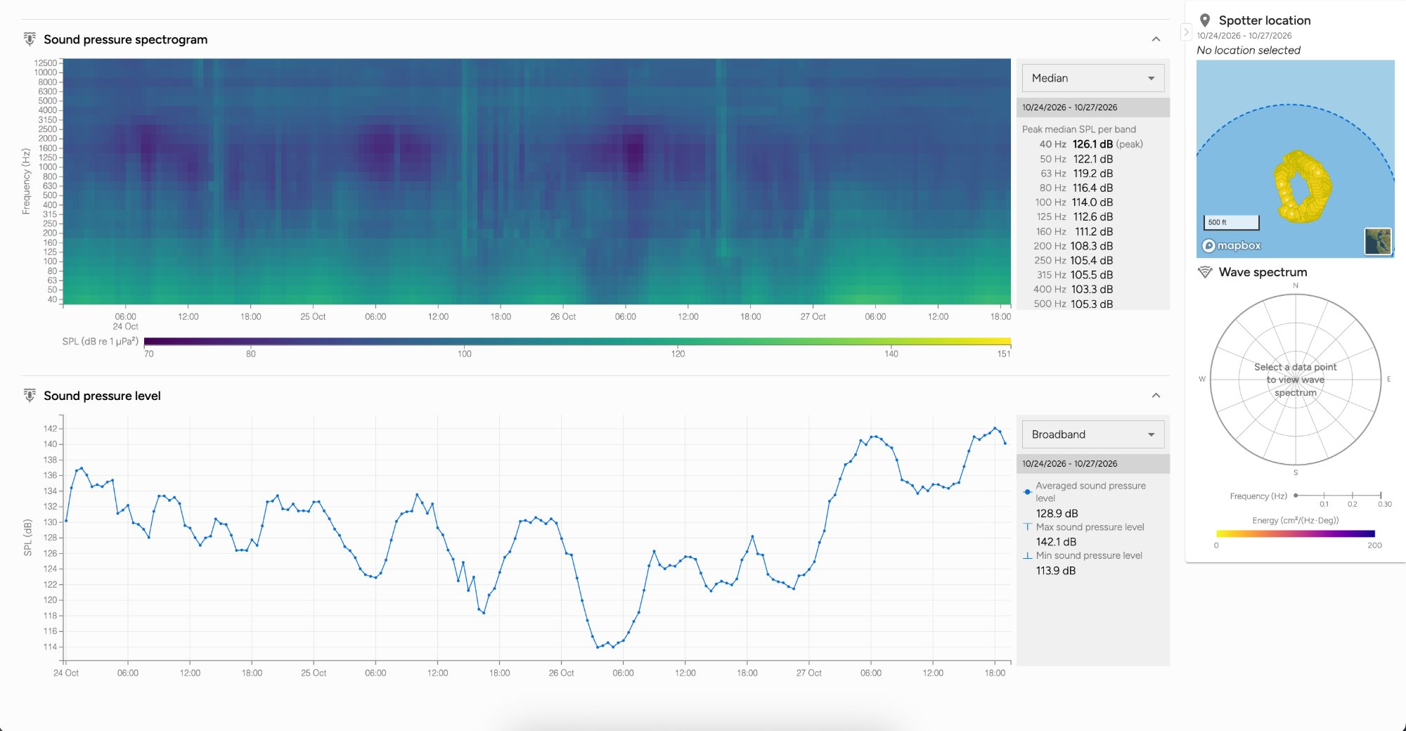
When a Spotter has a cellular connection, sending data costs far less. So, over cellular, we also send a one-second spectrogram: the level in each frequency band, every second.
In this case, the resolution is high enough to pick out individual events, like a ship passing, and to see exactly when they happened. Detection itself happens on the hydrophone, where models work from the full raw audio. More on that below.
One-second data also improves the coarser view. When we have it, we recompute each window's statistics from the one-second readings, at a resolution of about 0.025 dB, instead of using the compressed summary from the Spotter. For any slice of time, the dashboard shows the best data we have.
The complete recording stays with the instrument. It is written to the SD card on the hydrophone, and today, getting it means retrieving the card.
Soon, you'll be able to request short audio clips remotely, so hearing a moment of interest won't require a boat trip. Streaming raw audio around the clock is prohibitively expensive, but a short clip, fetched only when you ask for it, is far more manageable.
Clips will let anyone hear whether a detection sounds like what the detector claims. We'll be the first to use them that way: hearing the moments our detectors flag is one of the ways we make the detectors better.
Moving the data is half the job. The other half is making it legible on screen.
One problem took us a while: connecting a detection to the sound behind it. Lining detections up against the window statistics didn't help, since detectors work at a much finer resolution.
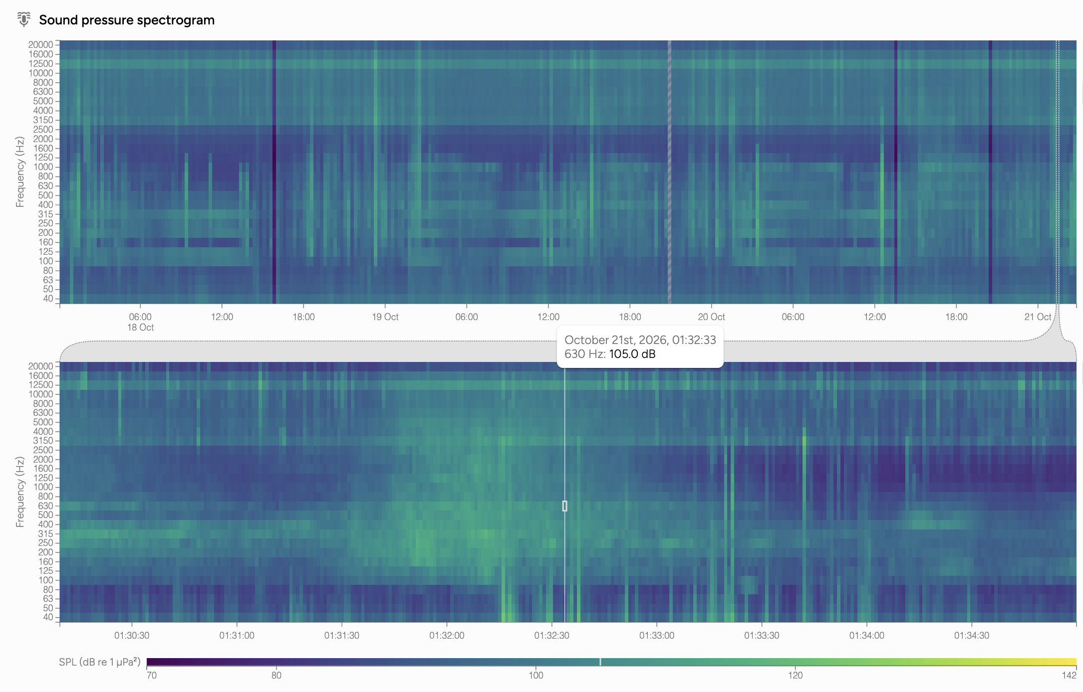
So now, when you click a detection in the dashboard, the one-second spectrogram folds out right beneath it: about fifteen minutes of context, with the 30 seconds the detector flagged highlighted, and curved lines tying the inset back to its spot on the parent chart. For a closer look at how we rebuilt the dashboard to keep up with sound, fetching only what's new each second instead of reloading everything, here's an episode of our Cool Stuff I Built series.
The connecting lines started as a debugging aid, so we could be sure the inset showed what we thought it showed. Once they were on screen, everyone wanted to keep them.
Everything in the dashboard, coarse and one-second alike, is also available through our sensor data API, so teams can pull acoustic data straight into their own tools and workflows.
Each layer above is a smarter way to send less data. The end point is to send almost none. If a Spotter in a remote marine protected area hears a fishing vessel, the most useful payload it can send isn't a spectrogram for someone ashore to interpret. It's a short message: there's a diesel-powered vessel here. A message that small is easy to send over satellite.
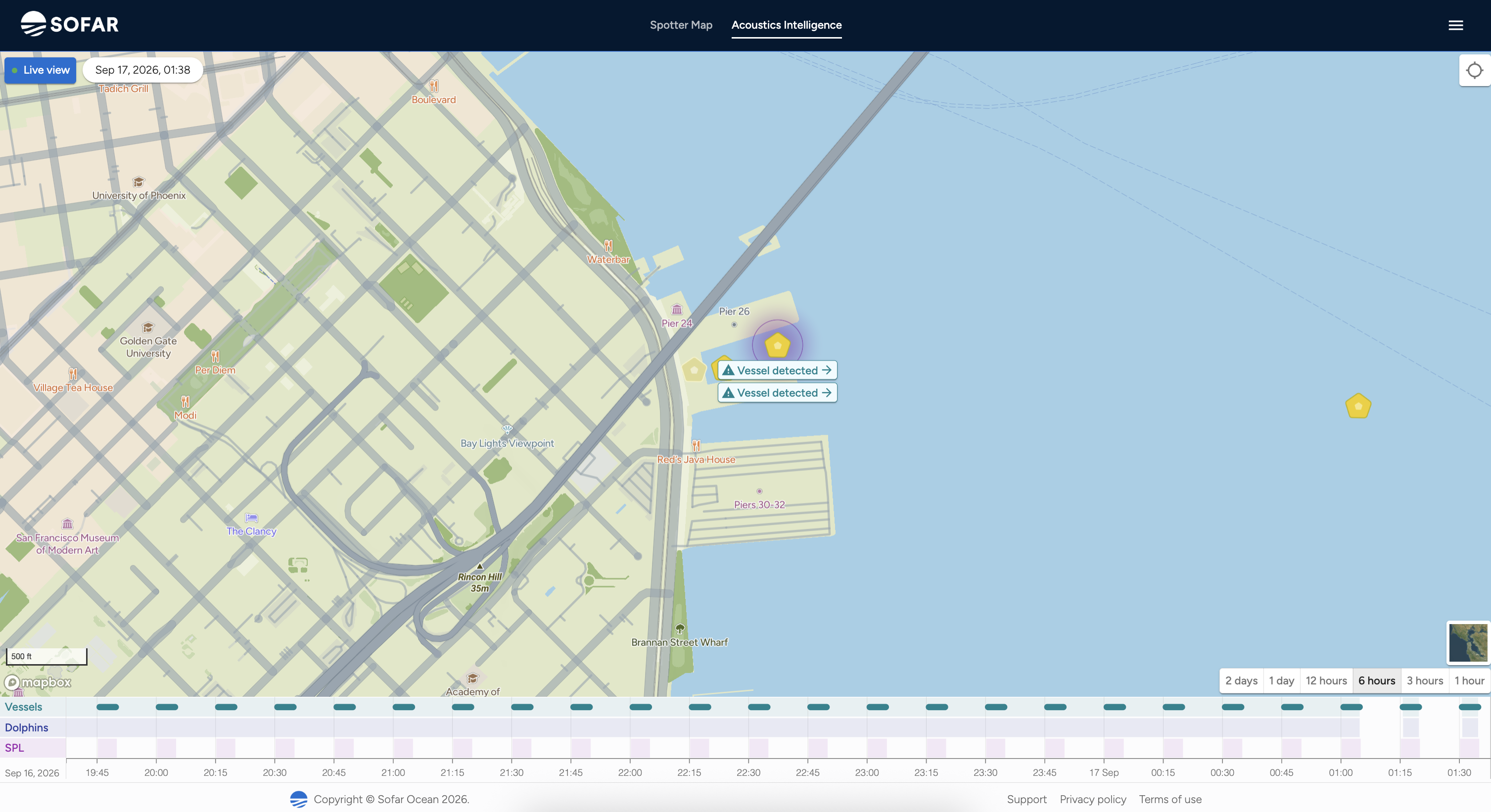
That means more of the processing happens on the device, and the hydrophone already carries a small Linux computer for exactly that. (Matt Krause covered how we made running it affordable on solar power.) We're building Spotter Sound as a platform for detectors, whether that's one of its prebuilt models or one of your own.
Further out is the question everyone eventually asks: not "did the Spotter hear something?" but "where is it?" Answering it means several Spotters comparing exactly when a sound reached each hydrophone, which makes timing the tricky part. GPS keeps every Spotter's clock in sync, so the work is making sure each sample is stamped the instant it's heard.
Even then, what each Spotter sends home is small: not the recording, just the moment it heard the sound. That's the pattern running through all of this. Every byte still counts, and the more a Spotter can work out on its own, the fewer of them it needs to send.